| Description: Wind Fields | Version: 9.0.0 | Updated: 08.11.16 | ||||||
Based on the generation of the 3D model in the preceding Terrain module, the simulation of the wind fields can now start. The wind fields are determined by solving the Reynolds Averaged Navier-Stokes equations (RANS). The standard k-epsilon model is applied as turbulence closure. Since the equations are non-linear the solution procedure is iterative. Starting with the initial conditions, which are guessed estimations, the solution is progressively resolved by iteration until a converged solution is achieved.
The flow variables that are solved are:
![]() Pressure (P1)
Pressure (P1)
![]() Velocity components (U1,V1,W1)
Velocity components (U1,V1,W1)
![]() Turbulent kinetic energy (KE)
Turbulent kinetic energy (KE)
![]() Turbulent dissipation rate (EP)
Turbulent dissipation rate (EP)
In more complex situations additional flow variables such as temperature (TEM1) can be included. Details on the physical background of this can be found in reports and publications on the WindSim web site.
Along the borders of the 3D model, information about the flow field must be supplied. These so called boundary conditions can be specified in two ways; either as analytical profiles or by nesting.
The analytical wind profiles are empirical profiles over flat terrain. The vertical profiles are dependent on the roughness height and if the temperature is activated also on the stability of the atmosphere. There are associated profiles for the turbulence. In case of a neutral atmosphere the wind profiles are log profiles. Applying the log profile along the border is equivalent to the placement of an infinite flat terrain upstream of the 3D model. This might be a bad assumption, therefore the results along the borders should be treated with care.
The nesting technique involves results from a former 3D model that fully covers the current 3D model. The profiles at the boundaries are interpolated from the former 3D model. This former model can be a WindSim model or a mesoscale meteorological model. Likewise the initial conditions are interpolated from the former 3D model.
Applying the nesting technique from a WindSim project reduces the inaccuracies introduced by applying the log profiles. It is highly recommended to start simulations in a large area and make refined models around the areas of interest using the nesting technique.
Using the nesting technique from a meteorological model gives the possibility of simulating special weather patterns. The information from the mesoscale model is interpolated to the WindSim grid as boundary and intial conditions. Meteorological data has to be given in an xyz_format and needs to be converted into the WindSim format dws. This can be done under Tools/Import mesoscale driving data. Up to know it is not possible to calculate the annual energy production from this simulations or to scale these results against climatologies. This needs to be done in own post-processing routines.
Be aware that 3D simulations can be a demanding on computer resources and time. Typically the simulation time is exponentially proportional to the number of cells in the model. It could be advantageous to split large models into smaller ones with the nesting technique.
Running several simulations simultaneously is not recommended.
For descriptions on the accuracy and convergence of the wind field simulations please refer to Accuracy and Convergence.
| Properties | ||||
| 1. Boundary and initial conditions | ||||
| Do nesting | ||||
| Specify whether nesting from a WindSim project or from a mesoscale meteorological model should be activated or not. Default value is False (-). | ||||
| Project file name | ||||
| Specify the name of the WindSim project as a .ws file. The nesting project must surround the current project, except at the upper boundary. If the vertical extension of the current project goes above the nesting project a constant extrapolation will be applied. Default value is none (-). | ||||
| Folder for mesoscale data | ||||
| Specify the folder name where the .dws files for this project are stored. The nesting project must surround the current project completely. | ||||
| Sectors for next run | ||||
| The wind fields will be simulated for the sectors given in this list. Any wind direction can be given, but if climatology data is then introduced, it is recommended to simulate the same sectors as those found in the climatology data. For further processing of the modules Wind Resources and Energy there must be a correspondence between the sectors in the climatology and the sectors for which flow simulations are performed. Sector 0 gives wind from North, sector 90 gives wind from East etc. Default values are 12 sectors from 0 to 330 (degrees). | ||||
| Cases for next run | ||||
| When nesting is done from a mesoscale meteorological model then the wind field will be simulated for the cases given in this list. Any case number until 1000 can be given. | ||||
| Height of boundary layer | ||||
| The log profile is defined from ground up to the boundary layer height, above this height the profile is constant. Default value is 500 (m). | ||||
| Speed above boundary layer | ||||
| The constant speed set above the boundary layer height. Default value is 10 (m/s). | ||||
| Use previous run as input | ||||
| If wind field simulation has been undertaken for a sector, the simulation can be continued by using the restart facility. Restart means that the solution from the former run is used for the initial conditions. In situations when the number of iterations specified in the preceding simulations have not led to a converged solution, a restart could progress the solution further towards convergence. The restart is not yet available for simulations with temperature included and for simulations driven by meteorological data. Default value is False (-). | ||||
| Boundary condition at top | ||||
| Two types of boundary conditions could be set at the top; a fixed pressure condition or a no-friction wall. The fixed pressure conditon could be used on complex terrain, while the no-friction wall is for use over flat terrain. Details on the behaviour of the top boundary condition can be found under Documentation on the WindSim web site. Default value is Fixed pressure. | ||||
| 2. Physical models | ||||
| Potential temperature | ||||
| Activation of the temperature equation. Depending on the type of initialization different boundary and initial conditions are set: | ||||
| Initialize from Monin-Obukhov length | ||||
| Depending on the given value for the Monin-Obukhov length the vertical profiles at the inlet are calculated stability dependend and a linear temperature gradient over the whole atmosphere is assumed. | ||||
| Reference temperature | ||||
| Potential temperature at sea level. Default value is 288 K. This value is only important for visualization purpose and does not influence the results. Select a value which is reasonable for your area. | ||||
| Monin-Obukhov length | ||||
| Stability Parameter with a range of -10000 to 10000 except 0. Default value is 100 m (very stable atmosphere). WindSim leaves the user the freedom to choose this parameter. Reasonable default values are |L|>1000 for neutral atmosphere, 200<L<1000 for stable atmosphere and 0<L<200 for a very stable atmosphere. 0>L>-200 for a very unstable atmosphere and -200>L>-2000 for an unstable atmosphere. As WindSim by default is setup to run steady state we do not recommend to run simulations with very unstable conditions as this can lead to divergence problems. | ||||
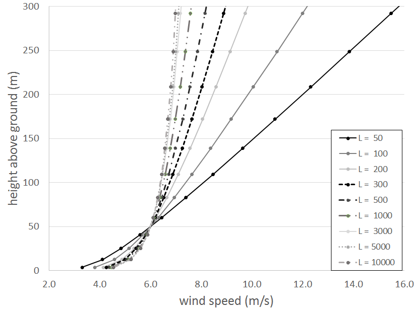
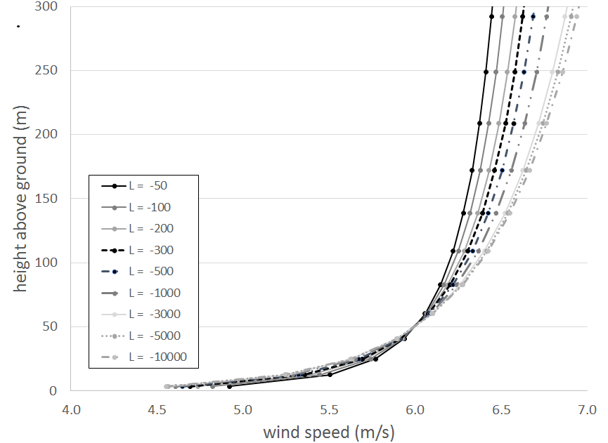
| Reference height and Wind Speed in reference height | ||||
| Depending on the stability of the atmosphere the wind profile in the higher elevations differs considerably (see figure 1). It is therefore more convenient to prescribe a “reference speed” in a “reference height” near the surface (e.g. mean annual wind speed of your climatology). This can be done by these two parameters which are 0 by default. If both values are set to zero the “speed at boundary layer height” is used to calculate the boundary profiles. The boundary layer height has to have a reasonable value as it defines the height where the TKE gets zero and the wind profiles get a constant value. For stable simulations we recommend to use a boundary layer height of around 300 m and for unstable simulations of around 800 m. | ||||
 |
||||
 |
||||
| Figure 1. Wind speed profile for different Monin-Obukhov lengths (roughness length of 0.001 m). | ||||
| Initialize from mesoscale | ||||
| The wind and temperature profiles at the boundaries and for initialization are interpolated from the mesoscale meteorological model. | ||||
| Turbulence model | ||||
| The default turbulence model is the standard k-ε model. The k-ε model belongs to the family of eddy viscosity models; an eddy viscosity, νt, is calculated by an analytical equation. A version with modified model constants is also available, please refer to the section "Presentations/Reports" at windsim.com for details. For high turbulent Reynolds numbers, the standard form of the k-ε model may be summarised as follows, with ,t denoting differentiation with respect to time and ,i denoting differentiation with respect to distance: | ||||
| (ρ k),t + (ρ Ui k - {ρ νt/PRT(k)} k,i ),i = ρ (Pk - ε) | ||||
| (ρ ε),t + (ρ Ui ε - {ρ νt/PRT(ε)} ε,i ),i = {ρ ε/k} (C1 Pk - C2 ε) | ||||
| νt = Cμ k2/ε | ||||
| Here k is the turbulent kinetic energy; ε is the dissipation rate; ρ is the fluid density; νt is the turbulent kinematic viscosity. Cμ,C1, C2, PRT(k), PRT(ε) are the model constants. | ||||
| Two further modifications of the k-ε model are available: the YAP correction [1] and the RNG (ReNormalization Group) version [2]. | ||||
| Air density | ||||
| This is the air density [kg/m3] used in the CFD simulations. | ||||
| Latitude | ||||
| Latitude given for the Coriolis force. | ||||
| 3. Calculation parameters | ||||
| Solver | ||||
| During the infancy of Computational Fluid Dynamics, only algorithms with small demands on computing power could survive. Computer memory was then extremely rare and expensive. In this context, use of the Patankar-Spalding SIMPLE algorithm and its descendants (SIMPLER, SIMPLEC, SIMPLEST, PISO...), based on the segregation of momentum and continuity equations was the best strategy to adopt. This strategy is activated with the segregated solver. | ||||
| But as the number of cells increases, the elliptic nature of the pressure field becomes a penalty and the global convergence of the method strongly slows down. The present state of the technology opens doors to other ways of thinking. The mean amount of RAM on PCs is continually increasing and its price decreasing so that, in many case, refining a grid up to the computer storage capability leeds to some huge CPU times to convergence. Therefore, as soon as the bottleneck becomes the required time for the solution, another velocity-pressure coupling strategy must be chosen. This is precisely the point with the coupled solver: an algebraic multi-grid solver which solves simultaneously the hydrodynamic variables in a whole-field manner. | ||||
| An increasing number of cells can also be handled by using the parallel solver. The solver makes it possible to split the simulation area into several domains which are calculated seperately. This speeds up the calculation process if several CPUs are available. | ||||
| Convergence problems can be overcome by using the General Collocated Velocity method (GCV). It solves the flow equations in body-fitted geometries in a way which differs from the PHOENICS-standard one in important respects. Distinguishing features of the GCV method are: 1) A block-structured multi-block formulation can be used and 2) GCV can handle highly non-orthogonal grids, being able to secure convergence with included angles as small as 10 degrees, which is much better then is achievable by the standard BFC formulation available via the segregated solver. | ||||
| Number of CPU's per sector | ||||
| The domain of each sector can be split into several subdomains which are calculated on different CPU's (1,2,4,8...). The number of simultaneous sectors times the number of CPU's per sector should not be higher then the total number of CPU's available. | ||||
| Number of simultaneous sectors | ||||
| Number of sectors which will be run simultaneously. The maximum number is limited to the number of CPU's of the machine. | ||||
| Number of iterations | ||||
| Number of iterations of the non-linear solution procedure. The number of iterations necessary to obtain a converged solution will depend on the number of cells. In particular this is true for the segregated solver, where models with more than 1 000 000 cells could require more than 1000 iterations to converge. The coupled solver will in general converge with less than 100 iterations even for larger models. Default value is 300 (-). | ||||
| Convergence wizard | ||||
| In cases where convergence is difficult to achieve, then the convergence wizard should be activated. The default convergence promoting procedure in WindSim based on so-called false time step relaxation is replaced by an automatic linear-under-relaxation set by the convergence wizard. The procedure will most probably give somewhat slower convergence; for the convergence wizard makes conservative rather than optimal choices. | ||||
| Convergence criteria | ||||
| The simulations can be stopped automatically when a certain level of convergence is reached. For this purpose the sums of absolute imbalances of the solved variables are calculated and then normalized by a reference value. If the normalized values fall below the given convergence criteria for all solved variables the simulation will stop. The default value is 5.E-3. | ||||
| 4. Convergence monitoring | ||||
| Coordinate system | ||||
| The spot value position is referenced to a local or global coordinate system. The local coordinate system has its origin in the lower left-hand corner of the 3D terrain model. The global system is the system specified in the grid.gws file. Default value is Local (-) | ||||
| Spot value X and Y position | ||||
| The spot value position is by default set to the centre of the terrain at ground level (nx/2,ny/2,1), where nx and ny is the number of cells in x and y-direction. The spot value position can be set anywhere in the horizontal plane. This allows monitoring of the development at points of special interest, like climatology and turbine positions. For details refer to Convergence. | ||||
| Field value to monitor | ||||
| The field value allows the user to choose a solved variable and follows the development of this variable as the solutions procedure progresses. The field variable is presented for the plane (nx,ny,1), where nx and ny is the number of cells in x and y-direction. With this information available it should be easier to introduce measures to ensure convergence even for very complex models. | ||||
| 5. Output | ||||
| Height of reduced wind database | ||||
| The results from the wind field simulations are stored in a compressed database consisting of flow variables, derived variables and auxiliary variables. In order to speed up the extraction of the data used in other WindSim modules a reduced database is also stored. In this database only the flow variables U1, V1, W1, KE are stored from the ground and up to the height specified herein. Default value is 200 (m). | ||||
| 6. Actuator disc | ||||
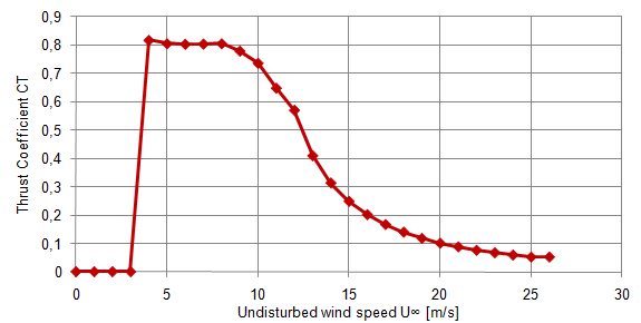
| The cells covering the swept area A exert forces direct against the wind, in the axial direction. The thrust of wind turbine does change with the wind speed according to the thrust coefficient curve provided by the manufacturer of the wind turbine. | ||||
 |
||||
| Figure 2. | Example of thrust coefficient curve. |
| Radial distribution | ||||
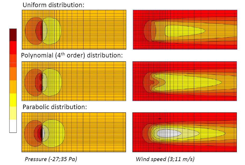
| Once the thrust at the turbine location is estimated, this can be distributed over the swept area in different manners. The axial forces in a wind turbine do change with the wind speed and are specific for each model of turbine according to the airfoils employed to design the blades. A realistic distribution of forces considers a peak of axial forces approximately in the mid-blade reducing to a lower value at the root and almost zero at the tip. Three distributions are chosen: a uniform distribution, a parabolic distribution (with a maximum value at the hub and zero at the tip), and a polynomial distribution (4th order with zero value at the tip, a maximum value at mid-span with a value that is half of the maximum at the hub position). | ||||
| Uniform dsitribution: | ||||
| t = T/A | ||||
| Parabolic dsitribution: | ||||
| t(ρ)=C1+C2 ρ2 | ||||
| Polynomial dsitribution: | ||||
| t(ρ)=C1+C2 ρ2+C3 ρ4 | ||||
| where: | ||||
| The radial position is given by ρ and the radius of the turbine's rotor is R. | ||||
 |
||||
| Figure 3. | Contour plots of pressure and wind speed at hub height with three types of radial distribution. |
| KE source | |||
| WindSim's actuator disc approach makes it possible to add a source of turbulence (source of turbulent kinetic energy) with a similar technique used to extract momentum. Since the aerodynamics of the turbine's rotor is not an actuator disc it is possible that the right amount of turbulence is not produced even if the right amount of momentum is extracted from the flow, hence the idea to manually adjust the turbulence production by the actuator disc. | |||
| The use of this option is suggested only to be employed by those with expertise in CFD codes and wind rotor aerodynamics. Competent users can use WindSim to tune the turbulence source Ck to match a more realistic generation of turbulence. | |||
| (ρ k),t + (ρ Ui k ),i = { [ρ νt/PRT(k)] k,i },i + ρ (Pk - ε) + Sk | |||
| where: | |||
| Sk is a source of turbulent kinetic energy per unit of volume [W/m3]. | |||
| Sk = Σ si / cell-volume | |||
| si = Ck ρ |u1,i|3 areai | |||
| where: | |||
| si is the source of KE per the i-th cell of the actuator disc. [W] | |||
| ρ is the air density. [kg/m3] | |||
| u1,i is the wind speed at the section of the rotor plane at the i-th cell of the actuator disc. [m/s] | |||
| areai is the area of the i-th cell of the actuator disc facing the wind directon. [m2] | |||
| Therefore Ck is a dimensionless group. | |||
| References | |||
| [1] | Yap, C. J. "Turbulent Heat and Momentum Transfer in Recirculating and Impinging Flows." PhD Thesis, Faculty of Technology, University of Manchester, United Kingdom, 1987. | ||
| [2] | Yakhot, V., Orszag, S.A., Thangam, S., Gatski, T.B. & Speziale, C.G. "Development of turbulence models for shear flows by a double expansion technique." Physics of Fluids A, Vol. 4, No. 7, pp1510-1520, 1992. | ||