| Description: Terrain | Version: 9.0.0 | Updated: 20.08.14 | ||||||
The first step in the set-up of flow field simulations, is the generation of a 3D model of the area of interest. This is done in the Terrain module. But first the basis for the 3D model must be available, which is a 2D dataset with elevation and roughness data in .gws format.
When starting a new project a grid.gws file is copied into the project. This file serves as a demo. The .gws format contains elevation and roughness data in a regular grid, the file can be viewed by using the Tools->View terrain model menu item.
Conversion from other formats is performed by clicking the Tools->Convert terrain model menu item. The Convert terrain model is subject to continuous development, so please contact WindSim AS if you need extensions in order to perform the conversion of your specific data, see examples of supported formats: third party formats Alternatively, you can convert your terrain model directly to the .gws format by using your own tools, see: terrain field data.
| Properties | |||
| 1. Terrain extension | |||
| Coordinate system | |||
| The coordinates in the grid.gws file can refer to any global orthogonal system. This coordinate system is called system 3 in the grid.gws file. After generation of the 3D model, a local coordinate system is introduced in the lower left-hand corner. Later in the Objects module the placements of objects can be referenced to by either the global or local coordinate systems. | |||
 |
|||
| Figure 1. | Coordinate system definition sketch. | ||
| X-range and Y-range | |||
| Extensions in the east-west direction and in the south-north direction. The specified coordinates may be increased to fit the nearest node in the grid.gws file, as interpolation of the underlying data is avoided. Default values are the minimum and maximum extensions in the grid.gws file (m). | |||
| Projection | |||
| Coordinate system of the global coordinate system. Giving Projection system, Datum, and Zone, WindSim calculates the EPSG code and stores that information in the grid.gws file for later use in WindPRO and Google export. | |||
| 2. Roughness | |||
| Roughness height | |||
| By default variable roughness heights are read from the grid.gws file. Alternatively a constant roughness height can be imposed in the model by specifying a non-zero value for the roughness height. | |||
| The roughness height is defined in the log-law: | |||
| U/Uτ = 1/κ ln(z/z 0) | |||
| where: | |||
| U = wind velocity | |||
| Uτ = friction velocity (τ0/ρ)0.5 | |||
| τ0 = shear stress | |||
| ρ = air density | |||
| κ = 0.435, von Karmans constant | |||
| z = coordinate in vertical direction | |||
| z 0 = Roughness height | |||
| 3. Numerical model | |||
| Refinement type | |||
| By default no refinement of the grid in the ground plane is performed. If a refinement area is specified, a denser distribution of nodes will be allocated within the refined area. The refined area is by default placed in the centre of the domain and the cell distribution is uniform within the refined area with an increasing cell size towards the borders. The data used for setting up the refinement area is stored in the current project under the folder dtm in the file simple_refinement.bws. Files with the extension .bws are blocking or refinement files. Finally .bws files can be loaded separately. | |||
| Refinement area, X-range and Y-range | |||
| Extensions in the east-west direction and in the south-north direction of the refinement area. By default the area is given in the centre with an extension equal to 1/3 of the total area extension. | |||
| Refinement/blocking file | |||
| Specification of a refinement or blocking file, syntax and examples. | |||
| Actuator disc | |||
| The actuator disc is the concept to model a turbine as a disc that is providing to the air flow forces supposed to be equivalent to the actual forces exchanged by a real wind turbine and the flow. With WindSim is possible to generate a grid modelling the wind turbines as a set of actuator discs. In order to design a computational grid with a set of actuator discs there is the need to set the Height above terrain, an object file (.ows) to define the layout of the wind farm and the number of spacings used to discretise the rotor diameter. | |||
| Height above terrain | |||
| The height above the terrain is defined as the vertical distance between the highest elevation point in the 3D model and the upper boundary. In order to set a proper value for this height, two seemingly contradictory requirements must be balanced. On the one hand, that the distribution of nodes in the vertical direction should be as dense as possible for obtaining accurate numerical solutions, in particular near the ground (see also Height distribution factor and Number of cells in Z direction). This requirement implies that the upper boundary should be placed as near the ground as possible. Yet, on the other hand, if the upper boundary is too close to the ground this would impose a blocking effect when the flow field passes over mountains. | |||
| As a rule of thumb the fraction between the minimum and maximum open area between the ground and the upper boundary, calculated as the model is traversed in west-east and south-north direction, should be lager than 0.95, i.e. (Open area Minimum)/(Open area Maximum) > 0.95. | |||
| By setting Height above terrain to Automatic a height will be calculated satisfying the relation (Open area Minimum)/(Open area Maximum) > 0.95. In some cases the automatic procedure might fail. The procedure will not capture the case with a ridge along the diagonal of the model, as the traverse in west-east and south-north direction will not detect significant changes in open area. But blocking might occur when the incoming flow is perpendicular to the ridge. Likewise for an isolated island or mountain the height of the upper boundary will be reduced as the total modelled area is increased, which could lead to blocking in extreme cases. | |||
| Alternatively a specific height could be given. | |||
| Object file | |||
| An actuator disc will be designed over each wind turbine. The layout of the wind farm is loaded from an object file (.ows). The same layout has to be loaded in the Objects module of WindSim, to reach the goal is useful to load the same object file in the Objects module. In order to run WindSim with the actuator disc option enabled, the module to be run after the Terrain module has to be the Objects (having the same layout included in the .ows of the Actuator disc), and, after the Objects, the Wind Fields. | |||
| Number spacings | |||
| The computational grid is designed having as reference length a subdivision of the rotor diameter wich will be therefore the minimum grid resolution, both horizontal and vertical, in the area of the wind farm. The grid will expand gradually from the wind farm region to the borders and top of the domain. The default value is 16 thas has proven to bring the discretization errors to an acceptable low value, therefore it is suggested to keep the number of spacings to 16 or higher. | |||
| Horizontal griding | |||
| Maximum number of cells | |||
| The 3D model will consists of nx*ny*nz cells. The number of cells in Z direction is set in Number of cells in Z direction. The number of cells in X and Y direction is set according to nx*ny*nz < maximum number of cells, by skipping nodes in the field data set. If Refinement is used then an interpolation is performed and the number of cells in the model will be approximately equal to the set maximum number of cells. Whenever a regular model is created then the extension of the model might be slightly modified as no interpolation of the underlying field data is performed, see figure 2. | |||
 |
|||
| Figure 2. | Field data extraction fitting the set maximum number of cells. In the upper case the maximum number of cells has been given a large value and the finest resolution possible for a regular grid model was created. In the middle case the maximum number of cells is smaller and the extraction procedure skipped every second node in the field data set. In the lower case refinement is set and the extraction procedure interpolates the field data set giving a model with approximately the maximum number of cells specified by the user. | ||
| The obtained number of cells and corresponding grid resolution is found under the 3D model section in the terrain report. The computing time required is exponentially proportional to the number of cells. Consider splitting a large model into several smaller models using the nesting technique, described under the Wind Field module, or to use the refinement technique. | |||
| Horizontal resolution | |||
| In the case of refinement described with a refinement area the computational grid can be constructed by assigning the Number of cells in the Z direction and the Horizontal resolution in the refined area, combined with a law for the expansion of the grid in the zones surrounding the refined area. | |||
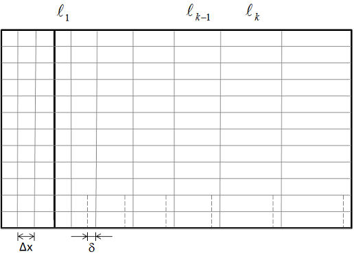
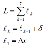
| Ratio additive length to resolution | |||
| The expansion of the grid is defined by the ratio of the additive length δ to the horizontal resolution set in the inner refined area. | |||
 |
|||
 |
|||
| Figure 3. | Expansion law, arithmetic sequence, for a zone on the right side of uniform grid. A fixed length δ is added to the length of a general cell k-1 to obtain the length of the successive cell k. The additive length δ is calculated from the Ratio additive length to resolution δ/Δx. | ||
| Height distribution factor | |||
| The cell distribution in the vertical direction follows an arithmetic sequence. The height distribution factor gives the fraction between the cell at the ground and the cell at the upper boundary. The vertical cell distribution could be inspected under the 3D model section in the terrain report. Default value is 0.1 (-). | |||
| Number of cells in Z direction | |||
| Number of cells in the vertical direction. Default value is 20 (cells). | |||
| Orthogonalize 3-D grid | |||
| Making the grid orthogonal is a technique for improving the convergence in cases with high inclination angles. By default the grid is not made orthogonal and then the grid extends in the vertical direction along straight vertical lines. Making the grid orthogonal means that the grid extends in the vertical direction along curved lines in an attempt of being perpendicular to the ground. In this way the cells will be less skewed in areas with high inclinations. When the inclination angles are higher than 50 ° it would be advisable to activate orthogonalization. The overall simulation time will go up when smoothing is activated. | |||
| The default setting is no orthogonalization. | |||
| 4. Smoothing | |||
| Smoothing Type | |||
| Various smoothing types can be used to smoothen the terrain. In some cases a wind field simulation fails to give a physical solution, the solution procedure diverges. Smoothing of the terrain is a technique for battling divergence. | |||
| Divergence could be caused by abrupt changes in the inclination between adjacent cells. Areas with abrupt changes in the inclination would be found in narrow valleys or at sharp mountain peaks. Typically, these areas would not be of interest for placing wind turbines, and as such a slight modification of the terrain could be accepted. | |||
| Terrain smoothing should be used with care, as excessive use will significantly change the heights of the terrain. Both the second order derivatives, which is a measure of the smoothness, and the changes between the original heights and the heights after smoothing are given in the report. Inspect these results, and make sure that areas of interest have not been significantly changed. | |||
| To smooth areas that are not of interest will speed-up the wind field simulations. | |||
| Bi-linear smoothing | |||
| Smoothens the terrain by marching along x and y directions sequentially. Bi-linear smoothing is a line smoothing routine. | |||
| Gaussian Smoothing | |||
| Smoothens the terrain by providing a Gaussian weighting to the neighboring nodes. Gaussian smoothing is a surface smoothing routine. In most cases, Gaussian smoothing will smoothen the terrain more than the Bi-linear smoothing. An example will be a saddle point, where the second order derivative is positive along one of the axis and negative along the other, which the Bi-linear smoothing might fail to smooth to the given Terrain smoothing limit. | |||
| Terrain smoothing limit | |||
| In mathematical terms changes in the inclination are represented by the second order derivatives of the elevation. On specifying a value for the Terrain smoothing limit, all places where the second order derivatives are higher than the smoothing limit are smoothed in an iterative procedure, until the second order derivatives are less than the specified limit. | |||
| Smoothing radius | |||
| The Smoothing radius is used to define the area where the smoothing is applied, in accordance with the below setting of Gradual smoothing type. The Smoothing radius is defined as the radius of a circle centered in the mid-point of the simulation domain. The Smoothing radius has a value between 0 and 1, reaching the value 1 at the corners of the simulation domain. | |||
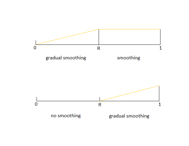
| Gradual smoothing type | |||
| The Gradual smoothing type is used to weight the smoothing in the inner or outer part of the simulation domain, preserving a continuous smoothing in the whole domain. The settings of the property variables Terrain smoothing limit, Smoothing radius and Gradual smoothing type allows for a wide range of terrain smoothing combinations. | |||
| Inner | |||
| Applies gradual smoothing from the center to the Smoothing radius and thereafter constant smoothing towards the border of the model, see definition sketch. | |||
| Outer | |||
| Applies no smoothing from the center to the Smoothing radius and thereafter a gradual smoothing towards the border of the model, see definition sketch | |||
 |
|||
| Figure 4. | Definition sketch for the Gradual smoothing type equal to Inner (top) and Outer (bottom), where R is the non-dimensional Smoothing radius. | ||
| 5. Forest | |||
| Forest | |||
| By default forest is disregarded. The forest model is activated by associating one roughness height present in the file grid.gws with the given forest characteristics, see below. | |||
| Roughness height | |||
| The roughness height used for specifying a forest. A forest is established at all locations with this given roughness height. | |||
| Forest height | |||
| The height of the forest. Default value is 30 (meters) | |||
| Forest porosity | |||
| The porosity of the forest. Allowed values between 0 and 1. A fully open area is obtained with porosity equal to 1, while porosity equal to 0 will give a fully blocked area. The porosity is not compatible with the GCV and parallel GCV solvers; it will be therefore disregarded if selected and CFD simulations run with the GCV solvers. | |||
| Forest resistive force constant C1 | |||
| The resistive force constant C1 is used to represent the forest as a resistive force proportional to the velocity, S1 = -ρ C1 U | |||
| Forest resistive force constant C2 | |||
| The resistive force constant C2 is used to represent the forest as a resistive force proportional to the velocity squared, S2 = -ρ C2 U|U| | |||
| Forest turbulence sources | |||
| Sources of turbulence are introduced in the KE and EP transport equations. Formally the model has been implemented as in Sanz (2003) [1] and Katul (2004) [2] with the model constants revised to be compatible with the default set of constants of the standard k-ε model. | |||
| Sk = C2 (βP|U|3 - βD|U|k) | |||
| Sε = C2 (Cε4 βP(ε/k)|U|3 - Cε5 βD|U|ε) | |||
| where: | |||
| βP = 1.0 | |||
| βD = 6.51 | |||
| Cε4 = 1.24 | |||
| Cε5 = 1.24 | |||
| The sources of turbulence will be applied only if the GCV or the parallel GCV is selected as Solver in the Wind Fields module. | |||
| Forest cell count in Z direction | |||
| The number of cells in the vertical direction used for the forest. The cell distribution is uniform. The remaining number of cells used above the forest, is Number of cells in Z direction - Forest cell count in Z direction. The vertical cell distribution could be inspected under the 3D model section in the terrain report. | |||
| References | |||
| [1] | Sanz, C. "A NOTE ON k - ε MODELLING OF VEGETATION CANOPY AIR-FLOWS." Boundary-Layer Meteorology, Kluwer Academic Publishers, No.108, pp191-197, 2003. | ||
| [2] | Katul, G.G., Mahrt, L., Poggi, D. & Sanz, C. "ONE- AND TWO-EQUATION MODELS FOR CANOPY TURBULENCE." Boundary-Layer Meteorology, Kluwer Academic Publishers, No.113, pp81-109, 2004. | ||